Summary:Constant propagation, as the name suggests, is to propagate the constant to the place where the constant is used, and replace the original variable with the constant.
This article is shared from HUAWEI CLOUD Community “Things About Compiler Optimization (2): Constant Propagation”, author: Bi Sheng’s assistant.
Basic knowledge inventory
- Basic Block:An instruction in a basic block, the processor will execute sequentially from the first instruction of the basic block to the last instruction of the basic block, without jumping to other places in the middle, and there will be no other places jumping to the basic block. Not the first command to come up.
- Control Flow Graph:The nodes of the control flow graph are basic blocks, and the edges represent jumps between basic blocks. There is an edge between basic block A and basic block B, indicating that the last instruction of basic block A is a jump instruction, which jumps to the first instruction of basic block B; or the last instruction of basic block A can be executed in sequence. Go to the first instruction of basic block B.
- SSA (Static Single Assignment):Static single assignment refers to a representation of a program in which a variable is assigned a value only once, and a new variable is used if the variable needs to be updated. To decide which branch variable to use, the Φ function is used.
E.g
min = a;
if(min > b)
     min = b;
return min;
Converted to SSA form as:
min = a;
if(min > b)
    min2 = b;
return Φ(min, min2)- Local optimization:Refers to the optimization of the basic block, cross-instruction.
- Global optimization:In-proc (function), optimization across basic blocks.
- Interprocedural optimization:Optimization across procedures (functions), compilation units.
1. What is constant propagation
First of all, let’s understand what constant propagation is. Constant propagation is also called constant folding, but some materials have different definitions of them. Let’s see what are they?
Constant propagation, as the name suggests, is to propagate the constant to the place where the constant is used, and replace the original variable with the constant.
->
What is constant folding? Constant folding is when the left and right sides of the operator are constants, the result is calculated to replace the original part of the expression.
–>
The current constant propagation optimization technology can realize the functions of propagation and folding described above at the same time, so they are usually not distinguished now. In this article, constant propagation and folding are collectively referred to as constant propagation.
Why are there constants?
There are 3 sources of constants in the program
- Written by programmers, such as magic number
- It is brought about by the expansion of the macro definition, which is very common in large project files
- Constants introduced by other optimization techniques during program optimization
Why Constant Propagation Optimization?
As can be seen from the above simple example, constant propagation can transfer the calculation originally at runtime to compile time, reducing the overhead of program runtime. At the same time, constant propagation also helps to achieve other optimizations, such as dead code elimination.
How to achieve?
The example of constant propagation introduced earlier is very simple and intuitive. If the control logic of the program is relatively complex, it is not a simple matter to determine whether a variable is a constant, and it is necessary to rely on the analysis of the data flow to determine whether a variable is a constant. And this judgment is conservative, that is, if a variable cannot be sufficiently proved to be a constant, it is considered a variable. This conservative analysis result is acceptable, because when we optimize the program, we prefer to ensure that the program semantics remain unchanged in the performance improvement and program semantic guarantee.
Let’s first learn about data flow analysis.
2. Data flow analysis
Data flow analysis is often an analysis technique to achieve global optimization, interprocedural optimization, or static analysis of programs. The information obtained from the analysis can support the implementation of various optimization techniques.
Consider the following instruction, what can we do to optimize it?
+ represents various valid operators, such as ±*/ etc.
Basically, there are three assumptions:
- If either x or y are constant, we can do constant propagation, replacing the variables x, y with constant values. If both x and y are constants, x+y can be calculated at compile time and assigned to z, so that such calculations will not be done at runtime.
- If x+y has been calculated before, and x and y have never been assigned (is a usable expression), then the value calculated last time can be directly assigned to z here, eliminating the need to calculate again The cost of such an optimization is called elimination of common subexpressions.
- If z is not used from here to the end of the program (z is an inactive variable), or if it is used, but is reassigned before use (z is an inactive variable), then this assignment statement is useless, you can Delete this statement.
It can be seen that for every possible optimization, a certain basis is required. These bases need to be obtained by analyzing the data flow.
Below we introduce three very basic data flow patterns.
- reach the fixed value
Tell us at a program point, where the variables in the procedure (function) are set (assigned). Commonly used in constant propagation, copy propagation. - Available expressions
Tell us what expressions are available at a program point. Commonly used in common subexpression elimination. - active variable
Tell us what are the active variables (variables that will be used in the future) at a program point. Often used to optimize register allocation and remove dead code.
2.1 Reaching the fixed value
2.1.1 Transfer function
Each statement in the program will have an impact on the state of the program. The state of the program includes the value of the register, the value of the memory, and the files read and written. For a particular data flow analysis, we only care about the parts that are useful for our analysis or program optimization. For example, for reaching fixed value analysis, we only track the fixed value of variables. For the analysis of available expressions, we track the generation of expressions and the assignment of expression components. For active variables, we care about the assignment and usage of variables.
We use transition functions to represent the effect of program statements on the program state:
OUT=f_d(IN)OUT=fd(IN)
f_dfd is the transition function of statement d. IN is the program state before statement d, and OUT is the program state after statement d.
Similarly, basic blocks have an effect on the program state, and basic blocks also have transition functions:
OUT = f_B(IN)OUT=fB(IN)
f_BfB is the transition function of the basic block B, and IN is the program state before the basic block B (it can also be expressed as IN[B]), OUT is the program state after the end of the basic block B (can also be expressed as OUT[B]).
Different analysis purposes have different transfer functions. For reaching fixed value analysis, if you encounter the following statement
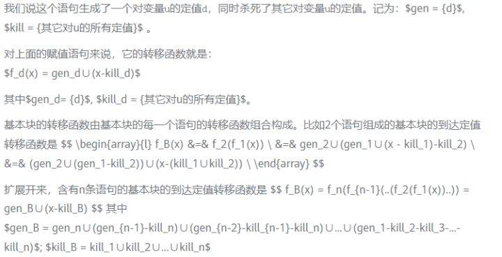
Let’s look at a specific example. In the flow graph below, the fixed value generated and the fixed value killed by each basic block have been marked on the right side of the figure.
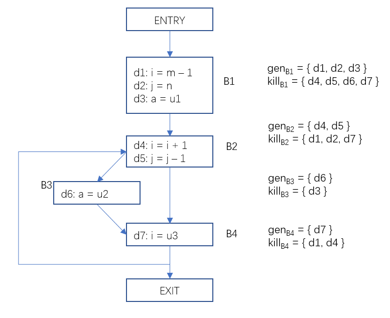
Figure 1 The generating set value and the killing set value set of the basic block
2.1.2 The basic idea of data flow analysis
For each basic block, according to the input state, apply the transition function, solve the output state, and repeat this operation until the output state of all basic blocks no longer changes.
2.1.3 meet operator
Figure 2 Data flow analysis – the meaning of the intersection operator
For the control flow graph above, the B2 precursor nodes include B1 and B2 themselves. The input state of B2 needs to be merged with the state OUT after the end of B1[B1] and the state OUT after B2 ends[B2], How to converge? This depends on the purpose of our analysis. For the arrival fixed value analysis, we need to collect the fixed value sets on all paths, so the union operation OUT is performed on the output of the predecessor node.[B1]∪OUT[B2]; For available expression analysis, we say that this expression is available on this basic block only when every path leading to this basic block has the generation of this expression, so the intersection operation is to find the intersection OUT[B1]∩OUT[B2]. The intersection operation is represented by the symbol ∧.
For the B2 basic block in the above control flow graph, in the first analysis, its own output is the initialized value ∅, and in the second analysis, its output is the output obtained after the previous analysis, it is possible It’s not ∅ anymore. After multiple iterations like this, its output doesn’t change anymore. When the outputs of all basic blocks are no longer changing, we say that this time has reached a fixed point (fix point).
When the analysis reaches a fixed point, the results of the data flow analysis are also obtained.
2.1.4 Iterative Algorithm for Reaching Fixed Value Analysis
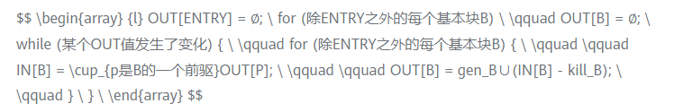
Description: This algorithm is an algorithm for reaching fixed value analysis on non-SSA representation. This relatively primitive algorithm is used here to introduce its most basic ideas; it will be more efficient to perform reaching fixed value analysis on SSA form. The prerequisite is that the program needs to be converted into a representation in SSA form. The active variable analysis, which is introduced later, is the same as the available expression analysis.
Program example
Next, we use a real program to perform a constant value analysis on the program represented by “Figure 1” (only the main program fragments are listed here)
// 定义一个基本块的属性结构
struct N{
    string name; // 基本块名称
 bitset gen {}; // 生成的定值
 bitset kill {}; // 杀死的定值
 bitset in {}; // 输入定值集合
 bitset out {}; // 输出定值集合
    vector pre{}; // 前驱基本块
};
 // 基本块的属性和初始化
 shared_ptr entry, b1, b2, b3, b4, exit{};
    entry = make_shared(N{"entry", 0, 0, 0, 0, {}});
    b1 = make_shared(N{"b1", 0B0000111, 0B1111000, 0, 0, {}});
    b2 = make_shared(N{"b2", 0B0011000, 0B1000011, 0, 0, {}});
    b3 = make_shared(N{"b3", 0B0100000, 0B0000100, 0, 0, {}});
    b4 = make_shared(N{"b4", 0B1000000, 0B0001001, 0, 0, {}});
    exit = make_shared(N{"exit", 0, 0, 0, 0, {}});
 // 构建基本块的前驱,形成CFG
    entry->pre = {nullptr};
    b1->pre = {entry};
    b2->pre = {b1, b4};
    b3->pre = {b2};
    b4->pre = {b2, b3};
    exit->pre = {b4};
 // 到达定值分析过程
    bool anyChange{};
    vector BBs{b1, b2, b3, b4, exit};
 do
 {
 anyChange = false;
 for (auto B : BBs)
 {
 for (auto p : B->pre)
 {
 B->in |= p->out;
 }
            auto new_out = B->gen | B->in & ~B->kill;
 if (new_out != B->out)
 {
 anyChange = true;
 }
 B->out = new_out;
 }
 } while (anyChange);
 // 输出每个基本块的输入定值,和输出定值
 for (auto B : BBs)
 {
 cout < < *B < < endl;
 }
Output result:
b1        0000000 1110000
b2        1110111 0011110
b3        0011110 0001110
b4        0011110 0010111
exit      0010111 0010111
The first column is the basic block name, the second column is the bit vector of the input fixed value set, and the third column is the bit vector of the output set.
In this way, we get the input fixed value set and the output fixed value set of each basic block. For example, for basic block B4, the bit vector <0011110> represents {d3,d4,d5,d6}, which is the set of arrival fixed values at the beginning of the basic block, and the bit vector <0010111> represents {d3,d5,d6,d7}, which is The set of arrival fixed values at the end of the basic block. With this information, it is easy to get at a certain program point p, which variables are set and where.
Feed the result back to the flow graph as follows:
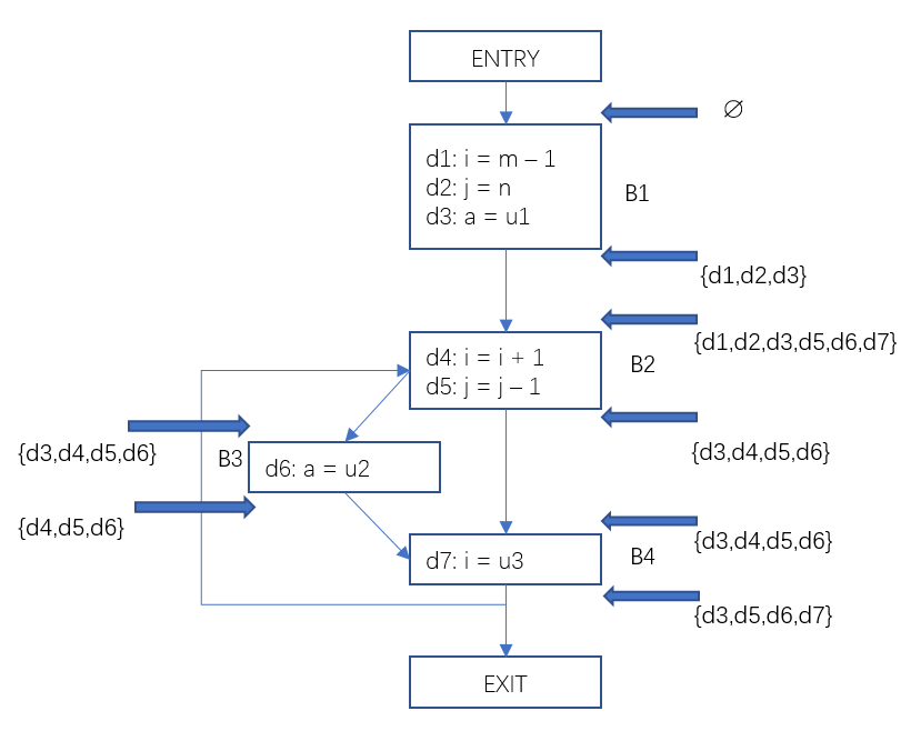
Figure 3 Data flow analysis – example of reaching a fixed value
Similarly, we can perform analysis of active variables, available expressions, in a similar way.
2.2 Active variables
A variable x is active at program point p, which means that the variable x is used on the path from program point p to the end of the program, and it is not newly assigned (not killed) before use.
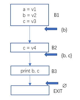
Figure 4 Data Flow Analysis – Active Variable Example 1
The only active variable at the exit of B1 is b, because variable a is never used again, and variable c is killed by the assignment in B2.
The active variables at the exit of B2 are b and c. Because only b and c are used in the following paths and are not reassigned before use.
Iterative Algorithm for Active Variable Analysis
Example
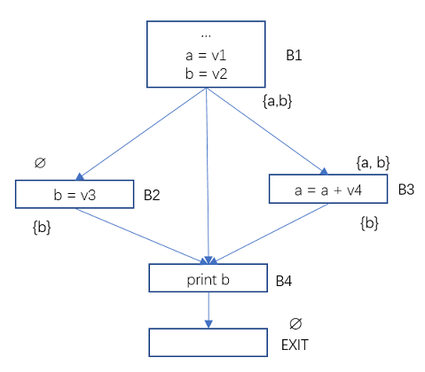
Figure 5 Data Flow Analysis – Active Variable Example 2
In the program flow diagram above, the Use and Def of the basic blocks B2, B3, B4 are:
Use[B2] = ∅, Def[B2] = {b}
Use[B3] = {a}, Def[B3] = {a}
Use[B4] = {b}, Def[B4] = ∅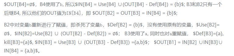
2.3 Available expressions
An expression is available if that expression has been evaluated on all paths to program point p, and the components of the expression have not been evaluated after evaluation.
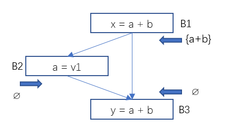
Figure 6 Data Flow Analysis – Example 1 of Available Expressions

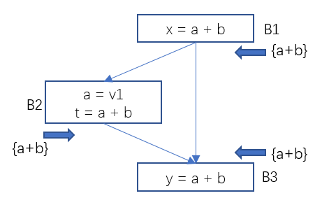
Figure 7 Data Flow Analysis – Example 2 of Available Expressions
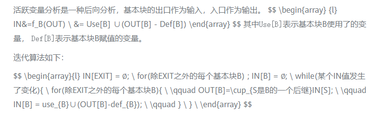
\qquad for(除ENTRY之外的每个基本块B)\{ \\

    \qquad \qquad IN[B]=\cap_{P是B的一个前驱}OUT[P]; \\

    \qquad \qquad OUT[B] = e\_gen_B∪(IN[B]-e\_kill_B); \\

\qquad \} \\
} \
\end{array} $$
3. Data flow analysis method of constant propagation
Introduced in front of the constant value analysis, active variable analysis, available expression analysis. They are very basic data flow analysis, and the results of these data flow analysis are used in many optimization processes. Now we come back to the optimization of constant propagation again. Constant propagation also requires analysis of data flow. It is very similar to reaching a constant value, but different because of the nature of constants.
3.1 Half-lattice used by constant propagation
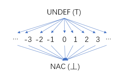
Figure 8 Constant Propagation – Half Lattice
Each variable in the procedure (function) has such a half-cell, and the value of the variable is the element in the half-cell. In the initial stage of constant propagation analysis, the values of all variables are uncertain, we use UNDEF (corresponding to the maximum value ⊤ in lattice theory); with our analysis, the values of some variables are constant, its value is It can correspond to an element in the middle row of the half grid, such as the constant 2. As the analysis proceeds, when the values of some variables are not constants (for example, the fixed values come from different precursors, and the fixed values of the variables in each precursor are different), it is represented by NAC (Not a Constant) at the bottom of the half grid (corresponding to The minimum value in lattice theory ⊥).
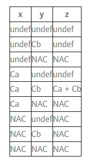
As mentioned earlier, the intersection operation is the merging of different sets. For constant propagation, the Meet Operator for each variable is the largest lower bound in a half-lattice of its different values. The rules for the intersection operation are as follows:
- UNDEF ∧ C = C (C represents a specific constant)
- UNDEF ∧ NAC = NAC
- C ∧ NAC = NAC
- NAC ∧ NAC = NAC
- C ∧ C = C
- C1 ∧ C2 = NAC (C1≠C2)
example:
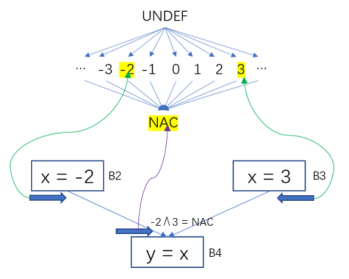
Figure 9 Constant Propagation – Variables Map to Half-Grid Values
The constant value of B2 for x is -2, and the value of B3 for x is constant 3. -2 ∧ 3 is taken on the half grid of the x variable.their maximum lower boundfor NAC.
3.2 Transfer Functions for Constant Propagation
For the statement z = x + y, the transition function is as follows:
For example, in the flow diagram below, the yellow markers represent variable states that have changed due to the influence of program statements. The variable x has the value 3 in the basic block B2, and the value in B3 is undef, and after their confluence (the largest lower bound) is the constant 3.
In B4, x is the constant 3, and x + 3 is the constant 6, so the instruction in B4 can be optimized to y = 6.
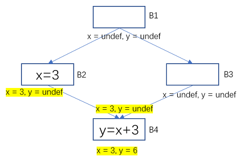
Figure 10 Example of constant propagation-transfer function
3.3 A Simple Algorithm for Constant Propagation
M[entry] == init
do
    change = false
    worklist < - all BBs; ∀B visisted(B) = false
 while worklist not empty do
 B = worklist.remove
 visited(B) = true
        m' = fB(m)
 ∀B' ∈ successors of B
 if visited(B') then
 continue
        end
 else
            m[B'] ∧= m'
 if m[B'] change then
                change = true
            end
 worklist.add(B')
        end
    end
while(change == true)
Example
The following program code
j = 1;
x = 10;
y = 1;
while(myRead()!=0){
    x = x * y;
    y = y * y;
    j = j + y;
}
p = j + x + y;
printf("%d\n", p);
its control flow graph
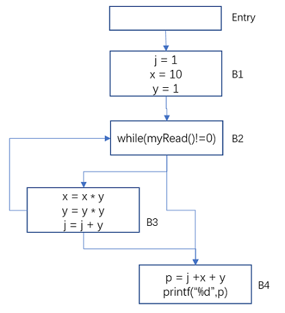
Figure 11 Constant Propagation – Example Control Flow Graph
Apply the above algorithm to this control flow graph
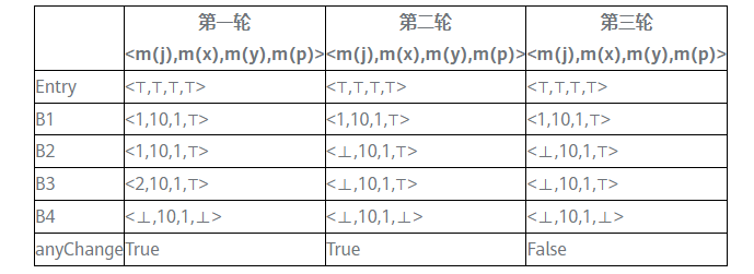
⊤ means undef, ⊥ means NAC (not a constant)
In the third iteration, the output of each basic block no longer changes and reaches a fixed point. It can be seen that at the exit of the basic block B3, only x and y are constants, which are 10 and 1 respectively, and j and p are non-constant.
Based on the above analysis, the above program can be optimized as follows
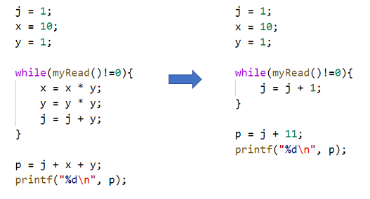
Figure 12 Constant propagation – the effect of program optimization
4. Bi Sheng and constant propagation in LLVM
Bi Sheng and LLVM’s SCCP is a relatively advanced constant propagation pass, and the algorithm it uses is Sparse Conditional Constant Propagation.
Its principle is similar to the above simple algorithm, with two differences:
- SCCP is an analysis performed on the representation of SSA. The constant propagation analysis is performed on the representation of SSA, which is faster than the analysis of the non-SSA representation, but the results are consistent.
- SCCP will judge the conditions in the conditional branch, distinguish which basic blocks are executable and which are not executable, which can remove the influence of the non-executable branch and make the constant propagation more accurate (reduce the situation that can be propagated but not propagated) .
Well, constant propagation is introduced here for everyone. Constant propagation involves the analysis of data flow, so this article also introduces data flow analysis and three common ideas of data flow analysis when introducing constant propagation.
5. References
Compilers Principles, Techniques, & Tools
http://www.cse.iitm.ac.in/~rupesh/teaching/pa/jan17/scribes/0-cp.pdf
Constant propagation with conditional branches https://dl.acm.org/doi/pdf/10.1145/103135.103136
Click Follow to learn about HUAWEI CLOUD’s new technologies for the first time~
#constant #propagation #compilers #Personal #space #HUAWEI #CLOUD #Developer #Alliance #News Fast Delivery