Summary:This case will take you to use an open source SMART dataset and the random forest algorithm in machine learning to train a hard disk failure prediction model and test the effect.
This article is shared from Huawei Cloud Community “Hard Disk Failure Prediction Based on Random Forest Algorithm”, author: HWCloudAI.
Experimental objectives
- Master the basic process of training models using machine learning methods;
- Master the basic methods of data analysis using pandas;
- Master the methods of using scikit-learn to construct, train, save, load, predict, statistical accuracy indicators and view confusion matrix of random forest models;
Case content introduction
With the development of the Internet and cloud computing, the demand for data storage is increasing day by day, and a large-scale mass data storage center is an essential infrastructure. Although new storage media such as SSDs have better performance than disks in many aspects, their high cost still makes most data centers unaffordable. Therefore, large data centers still use traditional mechanical Hard disk as storage medium.
The life cycle of mechanical hard drives is usually 3 to 5 years, and the failure rate increases significantly after 2 to 3 years, resulting in a sharp increase in the number of disk replacements. According to statistics, among server hardware failures, hard disk failures account for 48%+, which is an important factor affecting the reliability of server operation. As early as the 1990s, people realized that the value of data was far greater than the value of the hard disk itself, and longed for a technology that could predict hard disk failures and achieve relatively safe data protection, so SMART technology came into being.
SMART, the full name is “Self-Monitoring Analysis and Reporting Technology”, that is, “Self-Monitoring, Analysis and Reporting Technology”, which is an automatic hard disk status detection and early warning system and specification. Monitor and record the operating conditions of hard disk hardware such as magnetic heads, discs, motors, and circuits through detection instructions in the hard disk hardware, and compare them with the preset safety values set by the manufacturer. If the monitoring conditions will or have exceeded the expected If the safety range of the safety value is set, the monitoring hardware or software of the host computer can automatically warn the user and perform minor automatic repairs to ensure the safety of hard disk data in advance. Except for some very early hard drives, most hard drives are now equipped with this technology. For more introduction of this technology, please check SMART-Baidu Encyclopedia.
Although hard disk manufacturers use SMART technology to monitor the health status of hard disks, most manufacturers use fault prediction methods based on design rules, and the prediction effect is very poor, which cannot meet the increasingly strict demand for predicting hard disk failures in advance. Therefore, the industry expects to use machine learning technology to build a hard disk failure prediction model to more accurately detect hard disk failures in advance, reduce operation and maintenance costs, and improve service experience.
This case will take you to use an open source SMART dataset and the random forest algorithm in machine learning to train a hard disk failure prediction model and test the effect.
Theoretical knowledge about random forest algorithm,Can refer tothis video.
Precautions
- If you are using JupyterLab for the first time, please refer to “ModelAtrs JupyterLab User Guide” to learn how to use it;
- If you encounter errors when using JupyterLab, please refer to “ModelAtrs JupyterLab Common Problem Solutions” to try to solve the problem.
Experimental procedure
1. Dataset introduction
The dataset used in this case is an open source dataset from Backblaze, a computer backup and cloud storage service provider. Since 2013, Backbreze has publicly released the SMART log data of the hard drives used in their data centers every year, effectively promoting the development of hard drive failure prediction using machine learning technology.
Due to the large amount of SMART log data released by Backblaze, this case is a quick demonstration of the process of using machine learning to build a hard disk failure prediction model. Only the 2020 data released by the company is used. The relevant data has been prepared and placed in OBS. , run the following code to download this part of the data.
import os
import moxing as mox
if not os.path.exists('./dataset_2020'):
    mox.file.copy('obs://modelarts-labs-bj4-v2/course/ai_in_action/2021/machine_learning/hard_drive_disk_fail_prediction/datasets/dataset_2020.zip', './dataset_2020.zip')
    os.system('unzip dataset_2020.zip')

if not os.path.exists('./dataset_2020'):
    raise Exception('错误!数据不存在!')

!ls -lh ./dataset_2020
INFO:root:Using MoXing-v1.17.3-

INFO:root:Using OBS-Python-SDK-3.20.7
total 102M

-rw-r--r-- 1 ma-user ma-group  51M Mar 21 11:56 2020-12-08.csv

-rw-r--r-- 1 ma-user ma-group  51M Mar 21 11:56 2020-12-09.csv

-rw-r--r-- 1 ma-user ma-group 1.2M Mar 21 11:55 dataset_2020.csv

-rw-r--r-- 1 ma-user ma-group 3.5K Mar 22 15:59 prepare_data.py
Data Interpretation:
2020-12-08.csv: SMART log data on 2020-12-08 extracted from the 2020 Q4 dataset released by Backblaze
2020-12-09.csv: SMART log data on 2020-12-09 extracted from the 2020 Q4 dataset released by Backblaze
dataset_2020.csv: The processed SMART log data for the whole year of 2020. “Section 2.6 Category Balance Analysis” below will explain how to get this part of the data
prepare_data.py: Run this script, it will download the SMART log data for 2020 and process it to get dataset_2020.csv.Running this script requires 20G of local storage space
2. Data analysis
Before using machine learning to build any model, it is necessary to analyze the data set to understand the size of the data set, attribute names, attribute values, various statistical indicators, and null values. Because we need to understand the data before we can make good use of it.
2.1 Read csv file
pandas is a commonly used python data analysis module, we first use it to load the csv file in the dataset.Taking 2020-12-08.csv as an example, we first load the file to analyze the SMART log data
import pandas as pd
df_data = pd.read_csv("./dataset_2020/2020-12-08.csv")
type(df_data)
pandas.core.frame.DataFrame
2.2 View the scale of a single csv file data
print('单个csv文件数据的规模,行数:%d, 列数:%d' % (df_data.shape[0], df_data.shape[1]))
单个csv文件数据的规模,行数:162008, 列数:149
2.3 View the first 5 rows of data
After loading csv with pandas, you get a DataFrame object, which can be understood as a table. Call the head() function of the object to view the first 5 rows of data in the table.

5 rows × 149 columns
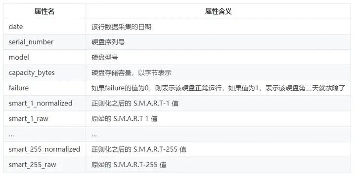
The above shows the first 5 rows of data in the table. The header is the attribute name, and the attribute value is below the attribute name. The backblaze website explains the meaning of the attribute value, and the translation is as follows:
2.4 View the statistical indicators of the data
After viewing the first 5 rows of data in the table, we call the describe() function of the DataFrame object to calculate the statistical indicators of the table data

8 rows × 146 columns
The above is the statistical index of table data. The describe() function performs statistical analysis on columns of numeric type by default. Since the first three columns of the table ‘date’, ‘serial_number’, and ‘model’ are string types, these three columns There are no statistical indicators.
The meaning of each row of statistical indicators is explained as follows:
count: how many non-null values the column has
mean: the mean of the column
std: the standard deviation of the column values
min: the minimum value of the column value
25%: 25% median value of the column value
50%: 50% of the median value of the column value
75%: 75% median value of the column value
max: the maximum value of the column value
2.5 View data null value
From the above output, it can be observed that the count index of some attributes is relatively small. For example, the count number of smart_2_raw is much smaller than the total number of rows of df_train, so we need to take a closer look at the null value of each column attribute and execute the following code You can check for empty values
df_data.isnull().sum()
date                         0
serial_number 0
model                        0
capacity_bytes 0
failure                      0
smart_1_normalized         179
smart_1_raw                179
smart_2_normalized      103169
smart_2_raw             103169
smart_3_normalized        1261
smart_3_raw               1261
smart_4_normalized        1261
smart_4_raw               1261
smart_5_normalized        1221
smart_5_raw               1221
smart_7_normalized        1261
smart_7_raw               1261
smart_8_normalized      103169
smart_8_raw             103169
smart_9_normalized         179
smart_9_raw                179
smart_10_normalized       1261
smart_10_raw              1261
smart_11_normalized     161290
smart_11_raw            161290
smart_12_normalized        179
smart_12_raw               179
smart_13_normalized     161968
smart_13_raw            161968
smart_15_normalized     162008
 ...
smart_232_normalized    160966
smart_232_raw           160966
smart_233_normalized    160926
smart_233_raw           160926
smart_234_normalized    162008
smart_234_raw           162008
smart_235_normalized    160964
smart_235_raw           160964
smart_240_normalized     38968
smart_240_raw            38968
smart_241_normalized     56030
smart_241_raw            56030
smart_242_normalized     56032
smart_242_raw            56032
smart_245_normalized    161968
smart_245_raw           161968
smart_247_normalized    162006
smart_247_raw           162006
smart_248_normalized    162006
smart_248_raw           162006
smart_250_normalized    162008
smart_250_raw           162008
smart_251_normalized    162008
smart_251_raw           162008
smart_252_normalized    162008
smart_252_raw           162008
smart_254_normalized    161725
smart_254_raw           161725
smart_255_normalized    162008
smart_255_raw           162008
Length: 149, dtype: int64
This display method is not very convenient for viewing. We draw the number of nullable values as a graph, which looks more intuitive
import numpy as np
import matplotlib.pyplot as plt
%matplotlib inline
df_data_null_num = df_data.isnull().sum()
x = list(range(len(df_data_null_num)))
y = df_data_null_num.values
plt.plot(x, y)
plt.show()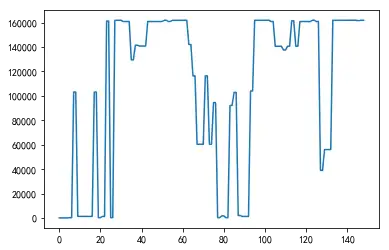
As can be seen from the above results, some attributes in the table have a large number of null values.
In the field of machine learning, it is very common to have null values in data sets. There are many reasons for null values. For example, there are many attributes in a user portrait, but not all users have corresponding attribute values. A null value is generated. Or some data is not collected due to transmission timeout, and null values may also appear.
2.6 Category Balance Analysis
The task we want to achieve is “hard disk failure prediction”, that is, to predict whether a certain hard disk is normal or damaged at a certain time. This is a failure prediction problem or anomaly detection problem. This kind of problem has a characteristic: there are many normal samples, There are very few failure samples, and the difference in the number of samples of the two types is very large.
For example, if you execute the following code, you can see that there are more than 160,000 normal hard disk samples in df_data, but only 8 faulty samples, and the categories are extremely unbalanced.
valid = df_data[df_data['failure'] == 0]
failed = df_data[df_data['failure'] == 1]
print("valid hdds:",len(valid))
print("failed hdds:",len(failed))
valid hdds: 162000
failed hdds: 8
Since the learning process of most machine learning methods is based on the idea of statistics, if you directly use the unbalanced data of the above categories for training, the ability of the model may be obviously biased towards samples with more categories and fewer categories. The samples will be “submerged” and will not play a role in the learning process, so we need to balance different types of data.
In order to obtain more fault sample data, we can select all fault samples from the 2020 annual SMART log data released by Backblaze, and also randomly select the same number of normal samples, which can be obtained through the following code accomplish.
This code has been commented out and requires 20G of local storage space to run.You don’t need to run this code, because dataset_2020.zip has been downloaded at the beginning of this case, and dataset_2020.csv is already provided in this compressed package. This csv is the file obtained by running the following code
# if not os.path.exists('./dataset_2020/dataset_2020.csv'):
#     os.system('python ./dataset_2020/prepare_data.py')
import gc
del df_data # 删除 df_data 对象
gc.collect() # 回收内存
2655
2.7 Loading a class-balanced dataset
dataset_2020.csv is the hard disk SMART log data that has been processed by category balance. Next, we load this file and confirm the category balance
df_data = pd.read_csv("./dataset_2020/dataset_2020.csv")
valid = df_data[df_data['failure'] == 0]
failed = df_data[df_data['failure'] == 1]
print("valid hdds:", len(valid))
print("failed hdds:", len(failed))
valid hdds: 1497
failed hdds: 1497
It can be seen that there are 1497 normal samples and fault samples
3. Feature engineering
After preparing the available training set, the next step is to do feature engineering. In layman’s terms, feature engineering is to select which attributes in the table to build a machine learning model. The quality of artificially designed features largely determines the quality of machine learning models, so researchers in the field of machine learning need to spend a lot of energy on artificially designed features, which is time-consuming, labor-intensive, and requires Engineering with expert experience.
3.1 Correlation research on SMART attribute and hard disk failure
(1) BackBlaze analyzed the correlation between its HDD failures and SMART attributes, and found that SMART 5, 187, 188, 197, 198 had the highest correlation rate with HDD failures, and these SMART attributes were also related to scan errors, reallocation counts related to trial count[1];
(2) El-Shimi et al. found that in addition to the above five features in the random forest model, there are five attributes of SMART 9, 193, 194, 241, and 242 that have the largest weight[2];
(3) Pitakrat et al. evaluated 21 machine learning algorithms for predicting hard disk failures, and found that among the 21 machine learning algorithms tested, the random forest algorithm had the largest area under the ROC curve, and the KNN classifier had the highest F1 value[3];
(4) Hughes et al. also studied machine learning methods for predicting hard disk failures. They analyzed the performance of SVM and Naive Bayesian. SVM achieved the highest performance, with a detection rate of 50.6% and a false positive rate of 0%.[4];
[1] Klein, Andy. “What SMART Hard Disk Errors Actually Tell Us.” Backblaze Blog Cloud Storage & Cloud Backup, 6 Oct. 2016, www.backblaze.com/blog/what-smart-stats-indicate-hard-drive-failures/
[2] El-Shimi, Ahmed. “Predicting Storage Failures.” VAULT-Linux Storage and File Systems Conference. VAULT-Linux Storage and File Systems Conference, 22 Mar. 2017, Cambridge.
[3] Pitakrat, Teerat, André van Hoorn, and Lars Grunske. “A comparison of machine learning algorithms for proactive hard disk drive failure detection.” Proceedings of the 4th international ACM Sigsoft symposium on Architecting critical systems. ACM, 2013.
[4] Hughes, Gordon F., et al. “Improved disk-drive failure warnings.” IEEE Transactions on Reliability 51.3 (2002): 350-357.
The above are some research results of the predecessors. This case plans to use the random forest model. Therefore, according to the research results of the second article above, SMART 5, 9, 187, 188, 193, 194, 197, 198, 241, 242 attributes can be selected As features, their meanings are:
SMART 5: Remap Sector Count
SMART 9: cumulative power-on time
SMART 187: Uncorrectable errors
SMART 188: Instruction timeout count
SMART 193: Head load/unload count
SMART 194: Temperature
SMART 197: Number of sectors waiting to be mapped
SMART 198: Errors reported to the operating system that cannot be corrected by hardware ECC
SMART 241: Total Logical Block Addressing Mode Writes
SMART 242: Total logical block addressing mode reads
In addition, since different models of hard drives from different hard drive manufacturers may have different standards for recording SMART log data, it is best to select the hard drive data of the same type as training data and train a model that predicts whether the hard drive of this type is faulty. If you need to predict whether multiple hard drives of different models fail, you may need to train multiple models separately.
3.2 Hard disk model selection
Execute the following code to see how much data is in each type of hard disk
df_data.model.value_counts()
ST12000NM0007 664
ST4000DM000 491
ST8000NM0055 320
ST12000NM0008 293
TOSHIBA MG07ACA14TA 212
ST8000DM002 195
HGST HMS5C4040BLE640 193
HGST HUH721212ALN604 153
TOSHIBA MQ01ABF050 99
ST12000NM001G 53
HGST HMS5C4040ALE640 50
ST500LM012 HN 40
TOSHIBA MQ01ABF050M 35
HGST HUH721212ALE600 34
ST10000NM0086 29
ST14000NM001G 23
HGST HUH721212ALE604 21
ST500LM030 15
HGST HUH728080ALE600 14
Seagate BarraCuda SSD ZA250CM10002 12
WDC WD5000LPVX 11
WDC WUH721414ALE6L4 10
ST6000DX000 9
TOSHIBA MD04ABA400V 3
Seagate SSD 2
ST8000DM004 2
ST18000NM000J 2
ST4000DM005 2
WDC WD5000LPCX 1
ST8000DM005 1
DELLBOSS VD 1
HGST HDS5C4040ALE630 1
TOSHIBA HDWF180 1
HGST HUS726040ALE610 1
ST16000NM001G 1
Name: model, dtype: int64
It can be seen that the ST12000NM0007 model has the largest amount of hard disk data, so we filter out the data of this type of hard disk
df_data_model = df_data[df_data['model'] == 'ST12000NM0007']3.3 Feature Selection
Select the 10 attributes mentioned above as features
features_specified = []
features = [5, 9, 187, 188, 193, 194, 197, 198, 241, 242]
for feature in features:
 features_specified += ["smart_{0}_raw".format(feature)]
X_data = df_data_model[features_specified]
Y_data = df_data_model['failure']
X_data.isnull().sum()
smart_5_raw      1
smart_9_raw      1
smart_187_raw    1
smart_188_raw    1
smart_193_raw    1
smart_194_raw    1
smart_197_raw    1
smart_198_raw    1
smart_241_raw    1
smart_242_raw    1
dtype: int64
There are empty values, so fill the empty values first
X_data = X_data.fillna(0)
print("valid hdds:", len(Y_data) - np.sum(Y_data.values))
print("failed hdds:", np.sum(Y_data.values))
valid hdds: 325
failed hdds: 339
3.4 Divide training set and test set
Use sklearn’s train_test_split to divide the training set and test set, test_size indicates the proportion of the test set, generally the value is 0.3, 0.2 or 0.1
from sklearn.model_selection import train_test_split
X_train, X_test, Y_train, Y_test = train_test_split(X_data, Y_data, test_size=0.2, random_state=0)
4. Start training
4.1 Build the model
After preparing the training set and test set, you can start to build the model. The steps to build the model are very simple, just call the RandomForestClassifier in the machine learning framework sklearn
from sklearn.ensemble import RandomForestClassifier
rfc = RandomForestClassifier()
There are many hyperparameters of the random forest algorithm. Building a model with different parameter values will result in different training effects. For beginners, you can directly use the default parameter values provided in the library, and have a certain understanding of the principle of the random forest algorithm. After that, you can try to modify the parameters of the model to adjust the training effect of the model.
4.2 Data Fitting
The process of model training, that is, the process of fitting training data, is also very simple to implement, and the training can be started by calling the fit function
rfc.fit(X_train, Y_train)
/home/ma-user/anaconda3/envs/XGBoost-Sklearn/lib/python3.6/site-packages/sklearn/ensemble/forest.py:248: FutureWarning: The default value of n_estimators will change from 10 in version 0.20 to 100 in 0.22.
 "10 in version 0.20 to 100 in 0.22.", FutureWarning)
RandomForestClassifier(bootstrap=True, class_weight=None, criterion='gini',
 max_depth=None, max_features="auto", max_leaf_nodes=None,
 min_impurity_decrease=0.0, min_impurity_split=None,
 min_samples_leaf=1, min_samples_split=2,
 min_weight_fraction_leaf=0.0, n_estimators=10, n_jobs=None,
 oob_score=False, random_state=None, verbose=0,
 warm_start=False)
5 start forecasting
Call the predict function to start predicting
Y_pred = rfc.predict(X_test) 5.1 Statistical prediction accuracy
In machine learning, there are four commonly used performance indicators for classification problems: accuracy (precision), precision (precision rate), recall (recall rate), and F1-Score. The closer the four indicators are to 1, the better the effect. it is good. There are functions of these four indicators in the sklearn library, which can be called directly.
Regarding the theoretical explanation of the four indicators,Can refer tothis video
from sklearn.metrics import accuracy_score, precision_score, recall_score, f1_score
print("Model used is: Random Forest classifier")
acc = accuracy_score(Y_test, Y_pred)
print("The accuracy is {}".format(acc))
prec = precision_score(Y_test, Y_pred)
print("The precision is {}".format(prec))
rec = recall_score(Y_test, Y_pred)
print("The recall is {}".format(rec))
f1 = f1_score(Y_test, Y_pred)
print("The F1-Score is {}".format(f1))
Model used is: Random Forest classifier
The accuracy is 0.8270676691729323
The precision is 0.8548387096774194
The recall is 0.7910447761194029
The F1-Score is 0.8217054263565892
Every time the random forest model is trained, different test accuracy indicators of the model will be obtained. This is due to the randomness of the training process of the random forest algorithm, which is a normal phenomenon. However, the prediction results of the same model and the same sample are determined and unchanged.
5.2 Model saving, loading, and re-prediction
model save
import pickle
with open('hdd_failure_pred.pkl', 'wb') as fw:
 pickle.dump(rfc, fw)
model loading
with open('hdd_failure_pred.pkl', 'rb') as fr:
 new_rfc = pickle.load(fr)
Model re-prediction
new_Y_pred = new_rfc.predict(X_test)
new_prec = precision_score(Y_test, new_Y_pred)
print("The precision is {}".format(new_prec))
The precision is 0.8548387096774194
5.3 View confusion matrix
To analyze the effect of the classification model, you can also use the confusion matrix to view it. The horizontal axis of the confusion matrix represents the categories of the predicted results, the vertical axis represents the category of the real label, and the values in the matrix grid represent the overlapping of the corresponding horizontal and vertical coordinates. Test sample size.
import seaborn as sns
import matplotlib.pyplot as plt
from sklearn.metrics import confusion_matrix
LABELS = ['Healthy', 'Failed']
conf_matrix = confusion_matrix(Y_test, Y_pred)
plt.figure(figsize =(6, 6))
sns.heatmap(conf_matrix, xticklabels = LABELS,
 yticklabels = LABELS, annot = True, fmt ="d");
plt.title("Confusion matrix")
plt.ylabel('True class')
plt.xlabel('Predicted class')
plt.show() 
6. Ideas for improving the model
The above content is a demonstration of the process of building a hard disk failure prediction model using the random forest algorithm. The accuracy of the model is not high. There are several ideas to improve the accuracy of the model:
(1) This case only uses Backblaze’s 2020 data, you can try to use more training data;
(2) This case only uses 10 SMART attributes as features, you can try to use other methods to build features;
(3) This case uses the random forest algorithm to train the model, you can try to use other machine learning algorithms;
Click to follow and learn about Huawei Cloud’s fresh technologies for the first time~
#Hard #Disk #Failure #Prediction #Based #Random #Forest #Algorithm #HUAWEI #CLOUD #Developer #Alliances #personal #space #News Fast Delivery